

This is a package for Non-Negative Linear Models. It implements a
fast sequential coordinate descent algorithm (nnls) for non-negative least square (NNLS)
and two fast algorithms for non-negative matrix factorization(nnmf).
The function nnls in R package nnls
implemented Lawson-Hanson algorithm in Fortran for the above NNLS problem.
However the Lawson-Hanson algorithm is too slow to be embedded to solve other problems like NMF.
The nnls function in this package is implemented in C++, using a coordinate-wise descent algorithm,
which has been shown to be much faster. nnmf is a non-negative matrix factorization solver
using alternating NNLS and Brunet's multiplicative updates,
which are both implemented in C++ too. Due to the fast nnls, nnmf is way faster
than the standard R package NMF.
Thus NNLM is a package more suitable for larger data sets and bigger hidden features (rank).
In addition. nnls is parallelled via openMP for even better performance.
This package includes two main functions, nnls and nnmf. nnls solves the following non-negative least square(NNLS)
argmin||y - x β||₂, s.t., β ≥ 0
where subscript 2 indicates the Frobenius normal of a matrix, analogous to the L₂ normal of a vector. While `nnmf` solves a non-negative matrix factorization problem likeargmin ||A - WH||₂² + η ||W||₂² + β Σ||h||₁², s.t. W ≥ 0, H ≥ 0
where `h` represents each column of `H`. Here `η` can used to control magnitude of `W` and `β` is for both magnitude and sparsity of matrix `H`.library(devtools)
install_github('linxihui/NNLM')library(NNLM);
data(nsclc, package = 'NNLM')
str(nsclc)## num [1:200, 1:100] 7.06 6.41 7.4 9.38 5.74 ...
## - attr(*, "dimnames")=List of 2
## ..$ : chr [1:200] "PTK2B" "CTNS" "POLE" "NIPSNAP1" ...
## ..$ : chr [1:100] "P001" "P002" "P003" "P004" ...
# create 5 meta-gene signatures, using only 1 thread (no parallel)
decomp <- nnmf(nsclc[, 1:80], 5, method = 'nnls', n.threads = 1, rel.tol = 1e-6)
decomp
## user system elapsed
## 5.747 4.420 6.377
## RMSE: 0.7334227
plot(decomp, 'W', xlab = 'Meta-gene', ylab = 'Gene')
plot(decomp, 'H', ylab = 'Meta-gene', xlab = 'Patient')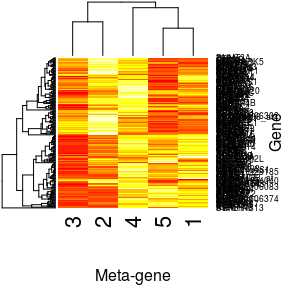

plot(decomp, ylab = 'RMSE')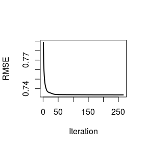
We see that the default alternating NNLS method coverage fairly quickly.
# find the expressions of meta-genes for patient 81-100
newH <- predict(decomp, nsclc[, 81:100], which = 'H', show.progress = FALSE)
str(newH)
## num [1:5, 1:20] 10 16.2 32.4 21.4 28.4 ...
## - attr(*, "dimnames")=List of 2
## ..$ : NULL
## ..$ : chr [1:20] "P081" "P082" "P083" "P084" ...
In micro-array data, the mRNA profile (tumour profile) is typically a mixture of cancer specific profile and healthy profile. In NMF, it can be viewed as
A = W H + W₀ H₁,
where `W` is unknown cancer profile, and `W₀` is known healthy profile. The task here is to de-convolute `W`, `H` and `H₁` from `A` and `W₀`.A more general deconvolution task can be expressed as
A = W H + W₀ H₁ + W₁ H₀,
where `H₀` is known coefficient matrix, e.g. a column matrix of 1. In this scenario, `W₁` can be interpreted as _homogeneous_ cancer profile within the specific cancer patients, and `W` is _heterogeneous_ cancer profile of interest for downstream analysis, such as diagnostic or prognostic capacity, sub-type clustering.This general deconvolution is implemented in nnmf via the alternating NNLS algorithm.
The known profile W₀ and H₀ can be passed via arguments W0 and H0. L₂ and L₁
constrain for unknown matrices are also supported.
# set up matrix
n <- 1000; m <- 200;
k <- 5; k1 <- 2; k2 <- 1;

set.seed(123);
W <- matrix(runif(n*k), n, k); # unknown heterogeneous cancer profile
H <- matrix(runif(k*m), k, m);
W0 <- matrix(runif(n*k1), n, k1); # known healthy profile
H1 <- matrix(runif(k1*m), k1, m);
W1 <- matrix(runif(n*k2), n, k2); # unknown common cancer profile
H0 <- matrix(1, k2, m);
noise <- 0.01*matrix(runif(n*m), n, m);

# A is the observed profile to be de-convoluted
A <- W %*% H + W0 %*% H1 + W1 %*% H0 + noise;

deconvol <- nnmf(A, k = 5, W0 = W0, H0 = H0);
## Warning in system.time(out <- switch(method, nnls = {: Target tolerence not
## reached. Try a larger max.iter.
Check if W and H, our main interest, are recovered.
round(cor(W, deconvol$W), 2);## [,1] [,2] [,3] [,4] [,5]
## [1,] -0.01 -0.03 1.00 0.00 0.08
## [2,] 0.98 0.06 -0.05 0.00 -0.05
## [3,] 0.21 -0.08 0.06 -0.17 0.99
## [4,] -0.01 1.00 0.00 0.05 -0.04
## [5,] -0.07 0.02 -0.05 0.99 0.04
round(cor(t(H), t(deconvol$H)), 2);## [,1] [,2] [,3] [,4] [,5]
## [1,] 0.03 0.02 1.00 0.17 0.09
## [2,] 0.99 0.02 -0.01 0.15 -0.02
## [3,] 0.22 -0.02 0.04 -0.06 0.98
## [4,] -0.02 1.00 0.05 0.01 0.03
## [5,] 0.09 -0.01 0.11 1.00 0.11
We see that W, H are just permuted. However, as we known that
the minimization problem for NMF usually has not unique solutions
for W and H. Therefore, W and H cannot be guaranteed to
be recovered exactly(different only with a permutation and a scaling).
permutation <- c(3, 1, 5, 2, 4);
round(cor(W, deconvol$W[, permutation]), 2);
## [,1] [,2] [,3] [,4] [,5]
## [1,] 1.00 -0.01 0.08 -0.03 0.00
## [2,] -0.05 0.98 -0.05 0.06 0.00
## [3,] 0.06 0.21 0.99 -0.08 -0.17
## [4,] 0.00 -0.01 -0.04 1.00 0.05
## [5,] -0.05 -0.07 0.04 0.02 0.99
round(cor(t(H), t(deconvol$H[permutation, ])), 2);## [,1] [,2] [,3] [,4] [,5]
## [1,] 1.00 0.03 0.09 0.02 0.17
## [2,] -0.01 0.99 -0.02 0.02 0.15
## [3,] 0.04 0.22 0.98 -0.02 -0.06
## [4,] 0.05 -0.02 0.03 1.00 0.01
## [5,] 0.11 0.09 0.11 -0.01 1.00
As from the following result, H₁, coefficients of health profile and
W₁, common cancer profile, are recovered fairly well.
round(cor(t(H1)), 2);## [,1] [,2]
## [1,] 1.00 0.16
## [2,] 0.16 1.00
round(cor(t(H1), t(deconvol$H1)), 2);## [,1] [,2]
## [1,] 1.00 0.15
## [2,] 0.16 1.00
round(cor(W1, deconvol$W1), 2);## [,1]
## [1,] 1
Assume S = {s_1, ..., s_L}, where s_l, l = 1, ..., L is a set of genes in sub-network s_l. One can
design W to be a matrix of l columns (or more), with W_{i, l} = 0, i not ∈ s_l. Then the matrix
factorization would learn the expression profile W_{i, l}, i ∈ S_l from the data. This is implemented
in nnmf with a logical mask matrix Wm = {δ_{i∈ s_l, l}}.
Since matrix A is assumed to have low rank k, information in A is redundant for the decomposition,
thus it possible to allow some entries in A absent. One can just use the non-missing entries to compute
W and H. Such methodology can be used to imputation the missing entries in A. This has an application
to only recomendation system. For example, in Netflix, each customer commends only a small proportion of
all the movies in Netflix and each movie is commended by some fraction of customers.
Thus the movie-customer comments (scores) matrix are fairely sparese (lots of missings).
Using a NNMF allowing missing values, one can predict the a customer's commends on a move he/she has not watched.
An recomendation can be done simply based on the predicted scores. In additon, the resulting W and H
can be used to further cluster movie and customer. This method is also implemented in nnmf when the input
matrix A has some missings.
This is obvious as the reconstruction from W and H lies on a smaller dimension, and should therefore give a smoother reconstruction. This noise reduction is particularly useful when the noise is not Gaussian which cannot be done using many other methods where Gaussian noise is assumed.
HeatmapExamplesVignetteTest.traivs.ymlcode coverageParallel, openMP supportSupport for missing values in NMF (can be used for imputation and recomendation system)- Add support for meta-genes: thresholding