Tensor Permeability is a C++ finite element (FE) framework and executable for the computation of full upscaled permeability tensors in porous media. It is based upon CSMP++ finite element data structures and algorithms. The main features of tensor permeability are:
-
Flow-based upscaling of the full permeability tensor for arbitrary geometries in porous media
- No assumptions are made on the orientation of upscaled permeability eigenvalues
- No periodicity requirements are made as to the underlying geometry and permeability distribution
- Emphasis on fracture support
-
Incorporation of locally varying and tensor-form permeability and transmissivity
- Matrix permeability and
- Fracture transmissivity can be input as full tensors (element-wise constant)
-
Highly tested against analytical solutions
- Numerous benchmarks, with emphasis on discrete fracture and matrix models (DFMs)
-
JSONbased application I/O, C++ API and Python interface.- Standardized file interfaces for application control and output
- C++ and Python API for seamless integration
This implementation is based on the JGR Publication Lang et. al, 2014, with the extension to locally tensorial element properties (anisotropic matrix permeability and fracture hydraulic aperture).
The tensor visualization script is based on a StackOverflow answer by unutbu
The volume averaging approach is based on a prototype developed by Siroos Azizmohammadi at University Leoben in 2012
- The binaries
tensor_permeability.exe,libamg_dyn.dll, andlibiomp5md.dll - MSVC runtime
And for models with more than 25000 elements
- Access to a SAMG license server (VPN, college network) and
OPTIONAL: For editing the settings files and visualization of VTU output we recommend
The command for the solver in the most basic case is
> tensor_permeability.exe
In which case the default settings file name settings.json is assumed to exits in the working directory.
The application will exit with a descriptive error message if the file is not present.
The command for reading a specific settings file is the same with the file name as added arguments
> tensor_permeability.exe case0_settings.json
In which case the settings file case0_settings.json is assumed to exits in the working directory.
The application will exit with a descriptive error message if the file is not present. The application can be called with
series of settings files, as so
> tensor_permeability.exe case0_settings.json case1_settings.json case2_settings.json
In which case all provided the settings files are assumed to exits in the working directory, and are run in order.
A minimal configuration looks like this:
	{
		"model":{
			"file name": "example",
			"format": "icem"
		},
		"configuration": {
			"matrix":{
				"configuration": "uniform",
				"permeability": 1.0E-15
			},
			"fractures":{
				"configuration": "uniform",
				"mechanical aperture": 0.0001,
				"hydraulic aperture": 0.0001
			}
		},
		"analysis":{
			"configuration": "uniform boundary distance",
			"distance": 2.0
		}
	}
Attention: Floating point values have to include a decimal value, i.e., we must write 1.0 and not 1.. This is a JSON
convention common in most parsers.
This settings file has three required subsections: model, configuration and analysis. An optional section output
will be introduced later. We're going to look at the model section first
The minimal model object loads a model from disk using a file name
	"file name": "example",
	"format": "icem" # supports: "icem" and "csmp binary"
For the icem option, the model is loaded from ANSYS Icem mesh, assuming example.asc and example.dat (binary mode)
present. In the above version of model, the model is loaded with all Icem families as csmp::Region, or csmp::Boundary.
An optional argument specifies a regions file to be used for the "format": "icem" case:
"regions file": "example"
In this case, the file example-regions.txt is assumed to be present in the woking directory and loaded as csmp regions file.
As an alternative option, a regions file can be generated for all regions specified in the configuration:
"regions": ["MATRIX", "FRACTURE_1", "FRACTURE_2", "TOP", "BOTTOM", "LEFT", "RIGHT", "FRONT", "BACK"]
This creates a temporary regions file that is being used when loading the Ansys model.
*Attention: Line element only Icem families will be removed automatically for 3D models, no need to specifiy regions just to exclude those.
In most cases, you'll be able to load the model as a whole without regions or regions file. *
Tensor Permeability internally uses tensorial material properties for local (element-wise constant) permability, hydraulic aperture, transmissivity and conductivity. Fracture mechanical aperture is a scalar property by definition. First, we will look at the simple case of isotropic properties.
Configuration refers to the initialization of material properties. Here, these properties are the matrix permeability, and the fracture mechanical and hydraulic aperture. The minimal configuration for both follows as:
	"matrix":{
		"configuration": "uniform",
		"permeability": 1.0E-15
	},
	"fractures":{
		"configuration": "uniform",
		"mechanical aperture": 0.0001,
		"hydraulic aperture": 0.0001
	}
In this case, all elements that qualify as matrix (volumetric elements) will be assigned a spherical permeability tensor
	1.0E-15 0.0     0.0
	0.0     1.0E-15 0.0       m2
	0.0     0.0     1.0E-15
And all fractures will have a spherical, in-plane projected tensor for the hydraulic aperture
	1.0E-3  0.0     0.0
	0.0     1.0E-3  0.0       m
	0.0     0.0     0.0
In this form of initialization, transmissivity and conductivity will be computed internally. Uniform values can also be assigned on a by-region basis. The configuration section then looks like
	"fractures":{
		"configuration": "regional uniform",
		"mechanical aperture": [0.0001, 0.0002],
		"hydraulic aperture": [0.0001, 0.00015],
		"fracture regions": ["FRACTURE_1", "FRACTURE_2"]
	}
This section specifies over what part(s) of the model the upscaled permeability tensors are to be evaluated. The most simple
set-up results in a single region omega that consists of all elements that keep a minimum distance to the boundary:
	"configuration": "uniform boundary distance",
	"distance": 5.0
Attention: For large models, this is expensive. Use the corner points box method below!
This constitutes the minimum settings. Running will, after application details, provide a summary like this
	Simulation Result Summary
	===========================

	omega
	-----
	Upscaled permeability tensor:
			  1.99e-15      -5.1e-19     -5.34e-16
			  -5.1e-19      2.97e-15      -1.2e-18
			 -5.34e-16      -1.2e-18      2.32e-15
	Upscaled permeability eigenvalues:
			  2.97e-15
			  2.71e-15
			  1.59e-15
Where omega refers to the sampling region created in the analysis settings above. The option uniform boundary distance is computationally expensive, but convenient for small models and verification
problems. Also, it creates only a single sampling region. A far better alternative, and more flexible, is to specifiy the box corner points of an arbitrary number of omega regions:
	"configuration": "bounding box",
	"corner points": [[[-3.0,-3.0,2.0],[3.0,3.0,8.0]], [[-2.0,-2.0,3.0],[2.0,2.0,7.0]]]
Now, two regions are evaluated, using the same pressure solution results. An arbitrary number of regions can be evaluated efficiently in this manner. The screen output now reads something like
	Simulation Result Summary
	===========================

	omega_0
	-------
	Upscaled permeability tensor:
			  1.04e-15     -6.82e-19      -1.7e-16
			 -6.82e-19      2.41e-15      5.48e-18
			  -1.7e-16      5.48e-18      1.72e-15
	Upscaled permeability eigenvalues:
			  2.41e-15
			  1.76e-15
			  9.99e-16

	omega_1
	-------
	Upscaled permeability tensor:
			  1.07e-15     -7.29e-19     -2.53e-16
			 -7.29e-19      3.45e-15      1.78e-18
			 -2.53e-16      1.78e-18      1.98e-15
	Upscaled permeability eigenvalues:
			  3.45e-15
			  2.04e-15
			     1e-15
For every omega that results from the above settings, eigenvalues and the full permeability tensor are output.
This optional section allows for output to files: Results as above and more to ascii (.json) and to VTK for visualization (.vtu).
A complete settings file so far including minimal visual and text output looks like this
	{
		"model":{
			"file name": "example",
			"format": "icem",
			"regions": ["MATRIX", "FRACTURE_1", "FRACTURE_2", "TOP", "BOTTOM", "LEFT", "RIGHT", "FRONT", "BACK"]
		},
		"configuration": {
			"matrix":{
				"configuration": "uniform",
				"permeability": 1.0E-15
			},
			"fractures":{
				"configuration": "regional uniform",
				"mechanical aperture": [0.0001, 0.0002],
				"hydraulic aperture": [0.0001, 0.00015],
				"fracture regions": ["FRACTURE_1", "FRACTURE_2"]
			}
		},
		"analysis":{
			"configuration": "bounding box",
			"corner points": [[[-3.0,-3.0,2.0],[3.0,3.0,8.0]], [[-2.0,-2.0,3.0],[2.0,2.0,7.0]]]
		},
		"output":{
			"results file name": "results.json",
			"vtu": true
		}
	}
The output section contains a complete description of available outputs:
	"results file name": "results.json",
	"vtu": true,
	"vtu regions": ["FRACTURE_1", "FRACTURE_2"]
A results summary will be written to results.json ("results file name": "results.json"), and visual outputs will be made for the entire model and all omega
regions ("vtu": true) and additionally for the regions "FRACTURE_1" and "FRACTURE_2" ("vtu regions": ["FRACTURE_1", "FRACTURE_2"])
For the FRACS2000 model Matthaei et al., 2005, a settings file that configures two sets of fractures looks like this:
	{
		"model":{
			"file name": "fracs2000",
			"format": "icem",
			"regions": ["TOP","BOTTOM","LEFT","RIGHT","FRONT","BACK","LIVE","FRAC_LIGHTBLUE","FRAC_GREEN"]
			},
		"configuration":{
			"matrix":{
				"configuration": "uniform",
				"permeability": 1.0E-15
			},
			"fractures":{
				"configuration": "regional uniform",
				"fracture regions": ["FRAC_LIGHTBLUE","FRAC_GREEN"],
				"mechanical aperture": [0.025, 0.01],
				"hydraulic aperture": [0.0075, 0.005]
			}
		},
		"analysis":{
			"configuration": "bounding box",
			"corner points": [[[700.0,20.0,500.0],[900.0,180.0,900.0]],[[100.0,20.0,100.0],[500.0,180.0,600.0]]]
		},
		"output":{
			"results file name": "results.json",
			"vtu": true,
			"vtu regions": ["FRAC_LIGHTBLUE","FRAC_GREEN"]
		}
	}
and produces a screen summary like so
	Simulation Result Summary
	===========================

	omega_0
	-------
	Upscaled permeability tensor:
			  8.84e-11      2.56e-12     -3.91e-11
			  2.56e-12      6.61e-10     -3.19e-11
			 -3.91e-11     -3.19e-11      2.13e-11
	Upscaled permeability eigenvalues:
			  6.62e-10
			  1.06e-10
			  2.12e-12

	omega_1
	-------
	Upscaled permeability tensor:
			  1.39e-10      3.82e-11     -4.94e-11
			  3.82e-11      8.78e-10       2.9e-12
			 -4.94e-11       2.9e-12      1.81e-10
	Upscaled permeability eigenvalues:
			  8.8e-10
			  2.13e-10
			  1.05e-10
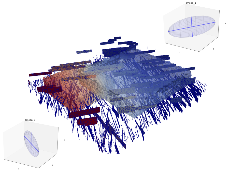
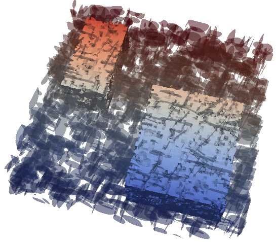
Visualization of the two sampling regions shows their location within the model
A complete account of the upscaling results is output in results.json:
	{
		"sampling regions": {
			"omega_0": {
				"eigen values": [
					2.11678759881574e-12,
					1.05955934709474e-10,
					6.62461357462325e-10
				],
				"eigen vectors": [
					[
						-0.411204005101016,
						-0.0424900717365861,
						-0.910552502600868
					],
					[
						0.911509395661833,
						-0.0277877804291414,
						-0.410339445921327
					],
					[
						-0.00786688051792995,
						-0.998710384977868,
						0.050156546215574
					]
				],
				"tensor": [
					8.84323457058634e-11,
					2.55802910081648e-12,
					-3.90993313778758e-11,
					2.55802910081648e-12,
					6.60839455644576e-10,
					-3.18938722898994e-11,
					-3.90993313778758e-11,
					-3.18938722898994e-11,
					2.12622784201741e-11
				]
			},
			"omega_1": {
				"eigen values": [
					1.04934242101843e-10,
					2.1309019227867e-10,
					8.79736614398485e-10
				],
				"eigen vectors": [
					[
						0.836994544415482,
						-0.0434672693426623,
						0.545482107052662
					],
					[
						0.544779026182029,
						-0.0276910553960627,
						-0.838122316898442
					],
					[
						-0.051535863734677,
						-0.99867101787673,
						-0.000502794367676158
					]
				],
				"tensor": [
					1.3909105056514e-10,
					3.82454558221439e-11,
					-4.93630065238251e-11,
					3.82454558221439e-11,
					8.7776151923872e-10,
					2.89918499323819e-12,
					-4.93630065238251e-11,
					2.89918499323819e-12,
					1.80908478975138e-10
				]
			}
		}
	}
and an ellipsoid visualization of the omega corresponding tensors looks like this for omega_0 and omega_2, respectively
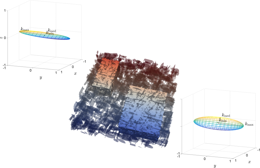
Lang, P. S., Paluszny, A., & Zimmerman, R. W. (2014). Permeability tensor of three-dimensional fractured porous rock and a comparison to trace map predictions. Journal of Geophysical Research: Solid Earth, 119(8), 6288-6307. doi:10.1002/2014JB011027
Matthaei, S. K., Geiger, S., Roberts, S. G., Paluszny, A., Belayneh, M., Burri, A., Heinrich, C. A. (2007). Numerical simulation of multi-phase fluid flow in structurally complex reservoirs. Geological Society, London, Special Publications, 292(1), 405-429. doi:10.1144/SP292.22