#canny-opencl This is an implementation of the Canny Edge Detection algorithm using OpenCL in C++. It uses OpenCV for some utility features, such as capturing an image from a webcam, opening/writing an image file, and converting from BGR to Grayscale. Note that it was considered outside of the scope of this project to maintain cross platform compatability, so it has only been tested in OSX 10.10. Additionally, because OpenCL applications can be heavily optimized (or broken) depending on the target hardware, the range of target hardware has been significantly limited. It was a goal to be able to utilize OpenCL on the CPU and GPU, so this does support both and contains optimized versions for both. While this should run on most modern macs, it has only been optimized and tested on the GPU and CPU of my early 2011 Macbook Pro 15".
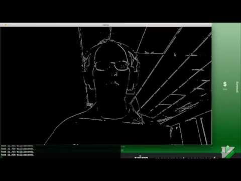
To see a short demonstration, view the link below:
#Table of Contents
#The Canny Edge Detection Algorithm As its name implies, the Canny edge detection algorithm finds edges in an image. The input is a grayscale image and the output is a black and white image with 1 pixel wide white lines denoting edges. An edge may be defined as place of high contrast. The rate at which the contrast changes indicates the strength of the edge. It has four stages: gaussian blur, sobel filtering, non-maximum suppression, and hysteresis thresholding. Below I will briefly discuss each stage.
##Gaussian Blur A gaussian blur is performed to reduce noise in the image. This is required because noise is generally high contrast and would thus lead to false positives. It is implemented using image convolution. For those unfamiliar with it, image convolution is an operation which essentially replaces each pixel with a weighted average of its neighbors. The weights chosen are very important and cause image convolution to be applicable to a number of problems. The gaussian blur weights closer pixels more heavily than distant ones.
##Sobel Filtering Sobel filtering replaces each pixel with a combination of the x and y derivatives of neighboring pixels. In doing so, pixels in high contrast areas will be "brighter" than pixels in low contrast areas. This essentially finds areas where edges are most likely to exist, but it does not pinpoint precisely where the edges are, so they exist as a gradient of probabilities. Similar to the gaussian blur, this is done using image convolution, but is performed twice: once for the x derivative and once for the y derivative. The pixel is then replaced with essentially: sqrt( (di/dx)^2 + (di/dy)^2 ) where di represents the change in intensity. During this stage, the direction of the gradient is also calculated for each pixel which is needed for non-maximum suppression.
##Non-Maximum Suppression At this point, there exists gradients representing probable edges, but our end goal is to represent edges as a single 1 pixel line. Non-maximum suppression rules out pixels which are part of an edge, but do not define the edge. The result is that we condense these wide gradient edges into a single 1 pixel line. Note that the result produced is still not the finished product, these lines are not purely white and don't necessarily indicate an edge, they instead still represent a probability of an edge. Non-maximum suppression is performed by using the direction of the gradient found in the previous stage and comparing the current pixel with neighboring pixels on either side. If the pixel is lower in intensity than ether of these neighboring pixels, then it is not considered be the true edge, so its value is replaced by 0. If the pixel is the highest intensity among its neighbors in the direction of the gradient, then it may be the true edge, so its value is retained.
##Hysteresis Thresholding We now have 1 pixel wide lines with values indicating the strength of the edge. In order to decide which of these should be considered an edge, we will use two threshold values. The low threshold indicates that pixels less than its value cannot be edges. The high threshold indicates that pixels higher than its value must be edges. Pixels between these values will only be edges if they neighbor an edge. The low threshold thus can be thought of as affecting the length of edges and the high threshold can be thought of as affecting the number of edges. Because of the definition, correct output of this stage cannot be found in one single pass examining only neighboring pixels, since a "maybe" edge can go either way. That said, an approximation may be made which gives vastly increased performance (since no edge traversal is needed) while keeping the output accuracy high enough for most applications. This implementation uses the approximation approach.
#Executables
It contains two executables: live-capture and benchmark-suite. Live capture
allows the user to view the results of canny edge detection in near real time
using the webcam as input. The benchmark suite uses several implementations
of the canny edge detection algorithm on multiple images. Each implementation
is run multiple times on each image. Next, the stages of the algorithm are
timed in isolation to better understand which steps are taking the longest.
##Building This has only been tested on a handful of similar machines and likely won't build on platforms other than OSX. If someone wishes to tweak it to work on linux and/or windows, I would gladly accept the pull request. Building and running is pretty easy and should be roughly the following:
$ ./tools/fetch-images.sh
$ mkdir build
$ cd build
$ cmake ..
$ make
$ cd ../bin
$ ./live-capture    # or ./benchmark-suite
#Code Layout The code is separated into three logical groups: image processors, live capture, and benchmarking.
##Image Processors All Image Processors are contained within the ImageProcessors namespace and inherit from the ImageProcessor abstract base class. Each image processor implements the canny edge detection algorithm, but each one does it in a different way. The focus of this project was canny edge detection in opencl, so the vast majority of effort was put into the OpenclImageProcessor class. Other image processors include SerialImageProcessor and CvImageProcessor.
###OpenclImageProcessor Based upon a boolean accepted by the constructor, this class can either target the CPU or GPU. When using the GPU, it will use 16x16 sized workgroups so that it may copy chunks of data to faster memory on the GPU and make fewer calls to global memory. While this is advantageous on the GPU, CPUs generally don't support two demensional work groups, so the same kernels cannot be used. As such, the kernels directory contains two sets. These kernels are only used for the OpenclImageProcessor.
###SerialImageProcessor The serial image processor was constructed by serializing the OpenclImageProcessor. It is used so that one may determine the speedup we get from using the OpenclImageProcessor.
###CvImageProcessor The Cv Image Processor simply uses OpenCV's canny edge detection algorithm. Unlike the other classes, it does not support executing the different stages of the algorithm in isolation.
##Live Capture usage: ./live-capture [cpu|serial] If no argument is given, live-capture will use the GPU.
An image processor is created based upon arguments if any exist. When operating in CPU and GPU mode, live-capture uses the OpenclImageProcessor. Live capture is performed using OpenCV to capture frames from the webcam. The frames are then fed into the image processor and its result is displayed on screen. The result is a near realtime video of canny edge detection algorithm running on the webcam's data.
##Benchmarking usage: ./benchmark-suite Note: This currently requires images to be fetched and on the local path ./images/. If you haven't already, run tools/fetch-images.sh to obtain these images.
Because the focus of this project was to produce a reasonably performant implementation of the canny edge detection algorithm, a fair amount of effort went into creating a flexible benchmarking system. It is desirable to know how this implementation compares to others, how it performs at different resolutions, and how much time each stage of the algorithm consumes. As such, the benchmarking-suite runs several iterations of each pair of image and implementation to find the mean and standard deviation of time taken. After benchmarking the full algorithm, each stage is run in isolation to capture the amount of time each stage consumes. The test images ranged in size from 0.3-288 megapixels.
#Optimization Methods Initially, a single set of OpenCL kernels were used that were intended to run on both the CPU and GPU. The performance on the CPU was better than expected; it gave 7x speedups over serial on a four core processor. However, the GPU performance was much lower than expected; it was slower than serial. The problem was pinpointed to redundant global memory accesses. Because most stages require that each pixel have knowledge of neighboring pixels, each pixel was retrieved 9 times or more from global memory. This access pattern is specifically what GPUs are weak at, so much of what should have been executed in parallel was being serialized by global memory accesses.
To solve this problem, two dimensional workgroups were used. Each work group copies pixel data to local memory which is much faster, but only accessible from within that workgroup. This reduced global memory accesses significantly and gave a 29x speedup over the previous version. The end result was 8-13x speedup over serial for the GPU, with peak performance for images that are approximately 10 megapixels. While running on the CPU, this implementation had a 7-10x speedup on images between 0.3-9 megapixels, but fell off very quickly for larger images.