Jeremy Newlin and Danny Rerucha

This repository contains the functionality for two types of acceleration structures. A uniform grid for accelerating nearest neighbor searches, and a KD Tree for accelerating ray tracking. Both are run on the GPU using CUDA. This project is a joint effort between Danny Rerucha and I for the GPU Programming Course at the University of Pennsylvania (CIS565).

Before we get to our discussion of the uniform grid, let's talk about nearest neighbor search for a second. It's hopefully somewhat clear what we're trying to accomplish - we want to find some neighboring particles (or photons, points in a cloud, etc) that fall within in a certain radius. This can be done pretty easily if performance is not a problem. You can simply loop over all of the particles and compare their distance with the radius. If the distance is less than the radius, you have a neighbor! For comparison purposes, we've included implementations of this algorithm in this project.

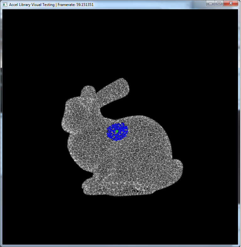An example of a particle (green) and its neighbors (blue).

But, we ARE interested in performance, and the naive solution isn't going to cut it. Enter the uniform grid, which is a type of spatial hashing data structure that allows for rapid nearest neighbor searches on the GPU (and CPU).

The basic idea of the structure can be described easily with a picture.

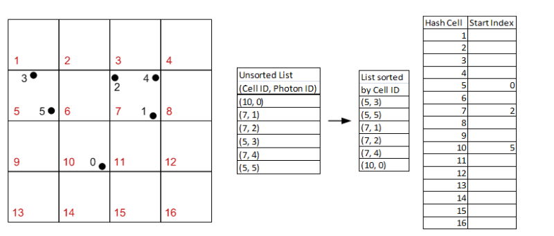
In this example, we can particles [0,1,2,3,4,5] in the grid. We hash the particles to their grid cell ids into an unsorted list. Then, we sort that list by grid cell id. Then, in the grid structure, we can simply store a single value - the index at which the grid cell start to contain particles in the sorted list.

So looking at Hash Cell 7 in the far right table, you can see that it has a value of 2. This means that grid cell 7 contains particles starting at index 2 in the sorted list. You can check to verify that this is indeed the case. Then, the next Hash Cell that stores a value is number 10 with a value of 5. You can then infer that Hash Cell 7 contains up to (but not including) index 5. That way, we know what particles each grid cell contains.

Now, how does this help speed up nearest neighbor search?

Remember that before we simply looped over the particles to find our neighbors. We're basically going to do the same thing here, but we've drastically reduced the number of particles we have to check. If you carefully choose the grid cell size to be the same as the radius of your search, you only have to check the surrounding grid cells for potential neighbors. By design any particle not within those cells will not pass the check of being less than the radius away from the current particle.

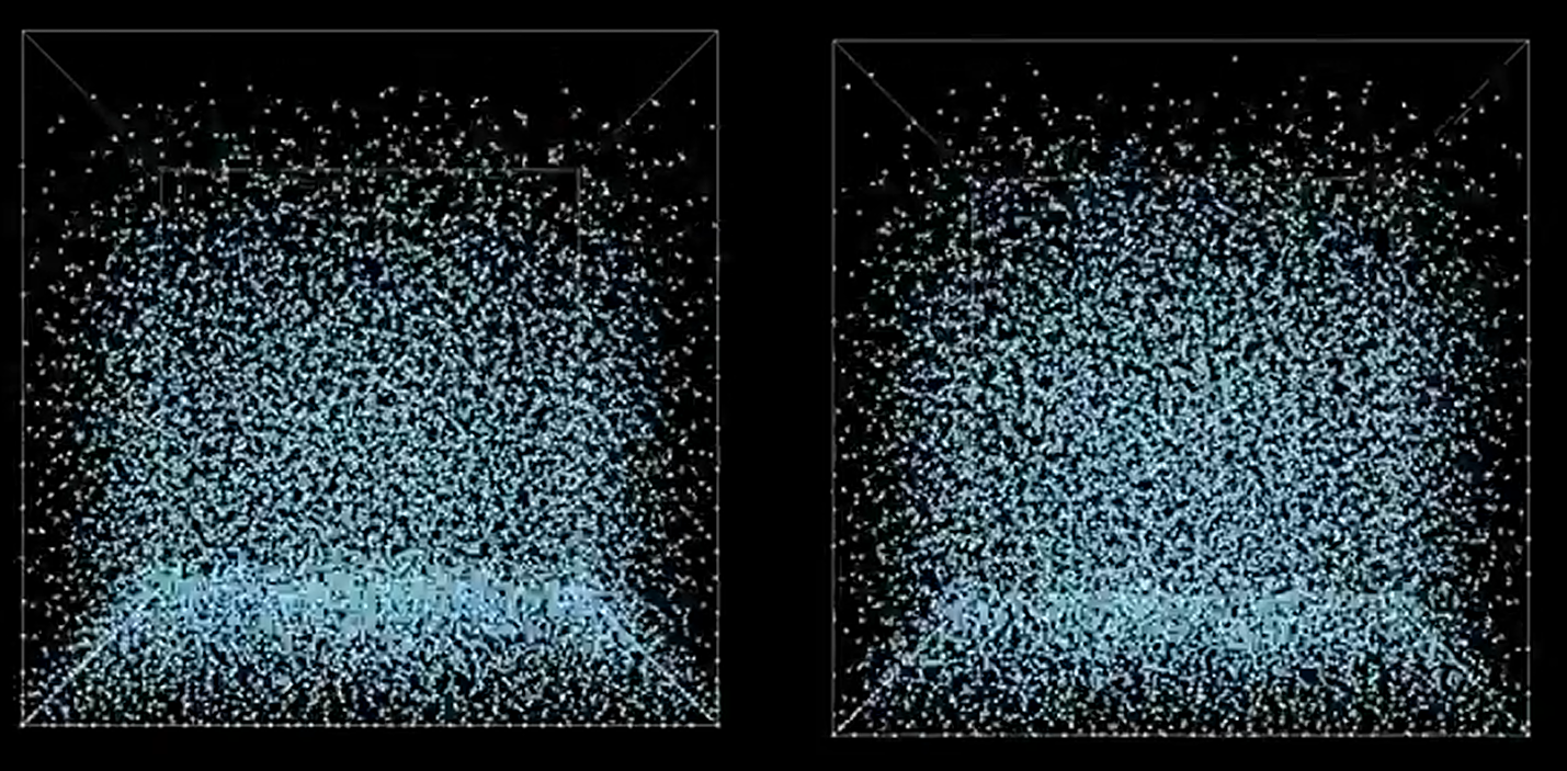
This image may be of use:

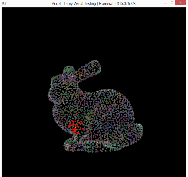
This is a visualization of the hashing step described above. Basically, particles in the same grid cell will be the same color in the image. So, instead of searching through the entire point set for neighbors, you can just look in your cell (and those around yours).

###Performance

And now time for some performance evaluations. First, we compared four different variations of the nearest neighbor search. With/without the grid, and on the GPU/CPU.

First, here's a comparison of how particle number (and density) and neighbor amount affect performance. Since that's a 3D data set, we got to make a 3D graph to show the results. Videos can be found by clicking on the images below.

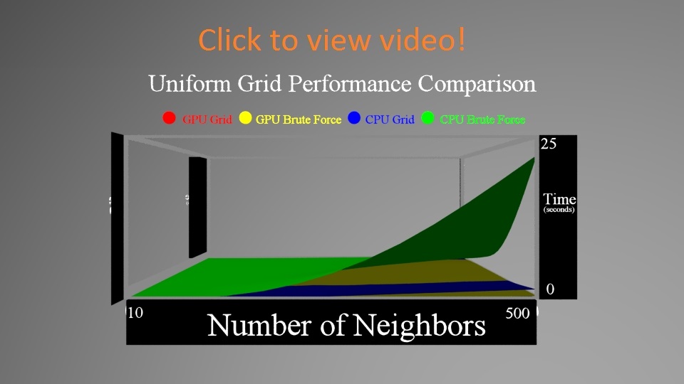
In the first video, you'll notice that the CPU brute force approach pops quite severely upwards as you increase both the neighbors and number of particles. The other 3 stay much lower (you can't even see the GPU grid graph even).

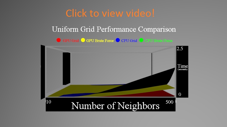
We zoom in on the data to look at the differences between the other 3. You'll notice that zoomed in you can see that the CPU Grid and GPU Brute Force Approaches do in fact get larger, while the GPU Grid stays flatter. Another interesting fact is that the CPU Grid sometimes outpaces the GPU Brute Force.

First, let's take a look at the two methods on the GPU - using the grid and brute forcing it.

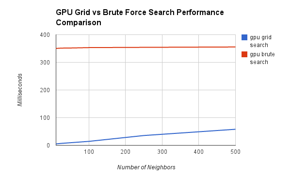
One interesting thing to note is that the the brute force stays relatively flat, while the grid is growing. This could be a problem when the number of neighbors you need approaches the size of your data set, or if your data set is highly dense. Our data set was relatively dense, and another important factor is sheer number of particles. This was on the order of 10,000 particles, which really is not that much. The brute force approach breaks down with many more particles (as seen in the videos above).

One other important metric we wanted to compare is how much overhead the grid is costing us. Clearly we're getting a net benefit from the grid structure, but we thought it would be interesting to quantify how much overhead we're paying for the speedup.

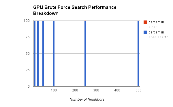
Clearly, in the brute force approach we're spending almost all of our time searching. We don't need to set anything up (the memory management is done once, and thus is omitted from the comparison).

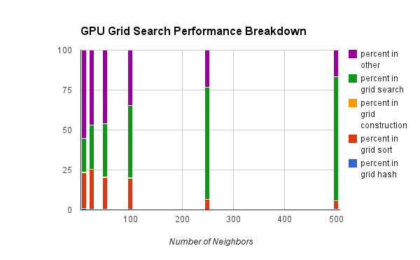
However, in the grid approach, we're spending a lot of time not searching. But that's a good thing! The entire point of this structure is to reduce the search time. The main costs here are the sorting step, and then the grid search. The purple "other" represents mostly error checking.

Finally, we have to look at the memory overhead that comes with building this grid. The cost of allocating the memory is amortized to 0, but we still need a sufficient amount of data to store the grid. The extra amount of data is a function of the grid cell size, and will be discussed below. The smaller the cell size, the greater the memory imprint. Our grid is built around being unit sized, so your radius should be sufficiently small for most applications to prevent dampening or other loss of fine grained detail.

At simulations with lower particle count on the order of 1000, the memory imprint is significant in terms of percentage at lower radii:

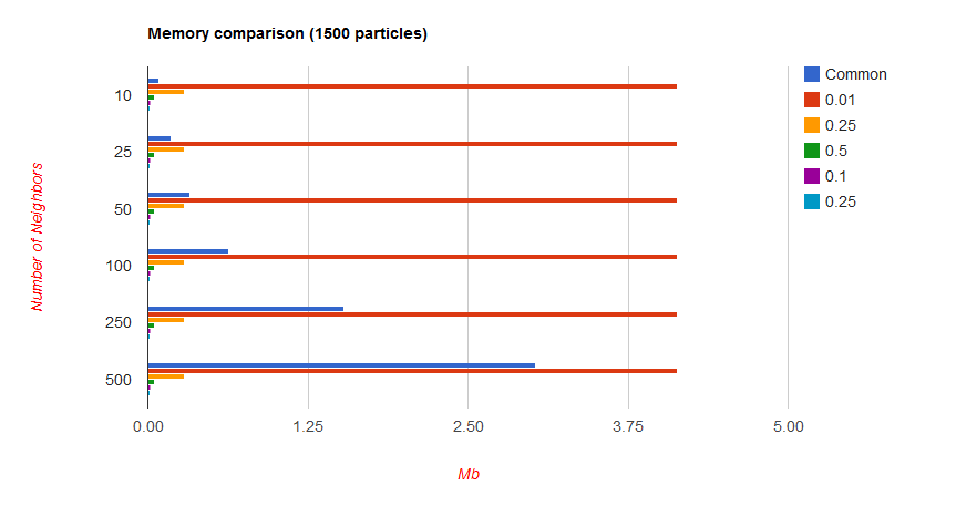
However, it is important to note that this is still only on the order of 5 extra Mb in the worst case.

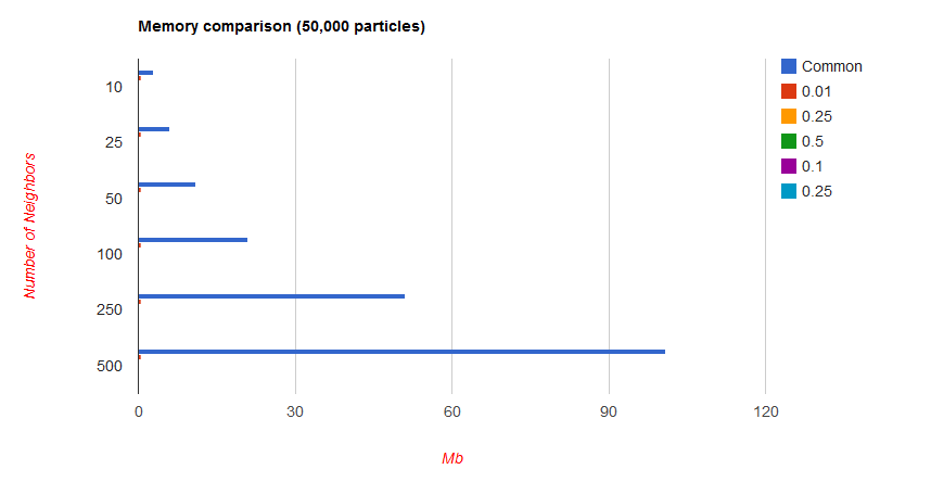
With higher particles counts, the extra memory becomes insignificant:

Overall, we're happy with grid - hopefully it will be of some use!

We put it to use in Jeremy's (kind of crappy) fluid sim. It definitely sped things up! With brute force search, the sim ran at just below 30 FPS, and with the grid, it ran at over 40 FPS. So 1.3x increase in speed. Not exactly revolutionary, but still pretty good. See the video below. (Unfortunately the only screen recording software we had access to was pretty bad, so you'll have to forgive the poor quality recording).

// Here is a code snippet to exemplify how to use the uniform grid.
#include "uniform_grid.h"
#include "mesh.h"

mesh m("\\path_to_file");
float h = 0.1f; //radius
glm::vec3 gridSize(1.0f/h, 1.0f/h, 1.0f/h);
hash_grid grid = hash_grid(m.numVerts, m.verts, gridSize);

int maxNumberOfNeighbors = 250;
bool useGPU = true;
bool useGrid= true;
grid.findNeighbors(maxNumberOfNeighbors , h, useGrid, useGPU);

for (int i=0; i<grid.numberOfPoints(); i+=1){
	int index = grid.getIndex(i);
	int numberOfNeighbors = grid.getNumberOfNeighbors(index);
	for (int j=0; j<numberOfNeighbors; j+=){
		// Get jth neighbor of particle i
		int neighborIndex = grid.getNeighbor(index, j);
		//Do something with this neighbor! 
	}
}

Next up, we have a KD Tree acceleration structure for ray tracking.

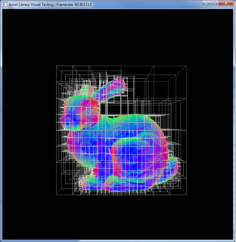
Similar to the uniform hash grid, this structure partitions the space into regions. In this case, each cell of the tree contains a set of triangles of the mesh. This is useful for ray tracking because when you want to intersect the mesh, you can use the tree structure to reduce the total number of intersections you have to compute. Let's examine the bunny mesh without the KD Tree.

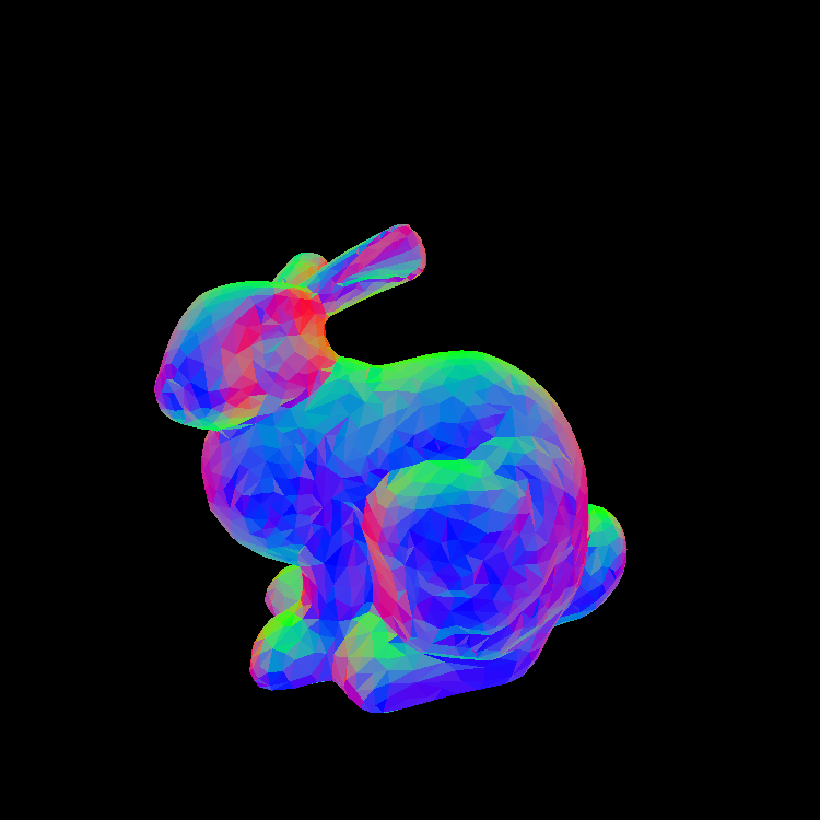
Now, the general case for intersecting this mesh using ray tracking is to simply loop over all of the triangles, finding the one that is the closes to the origin of the ray. Pretty simple but has one glaring problem. What about all of the pixels that have no chance of intersecting any triangle on the mesh? That's the majority of the image! We want to cull out those pixels and not even attempt ray tracking against the mesh. The easiest way to do that is to first try intersecting the bounding box of the mesh. If the ray doesn't hit that, there is no way that it could intersect a triangle on the mesh.

Now, you can think of a KD Tree as a set of bounding boxes of regions of the mesh. Then we just arrange them in a fancy way that helps us accelerate this process. The visualization below shows the number of ray-triangle intersections calculate at each pixel. Green represents no intersections, while red indicates the max number of intersections.

Max number of intersections - 29808. No acceleration structure at all - every pixel intersects every triangle.

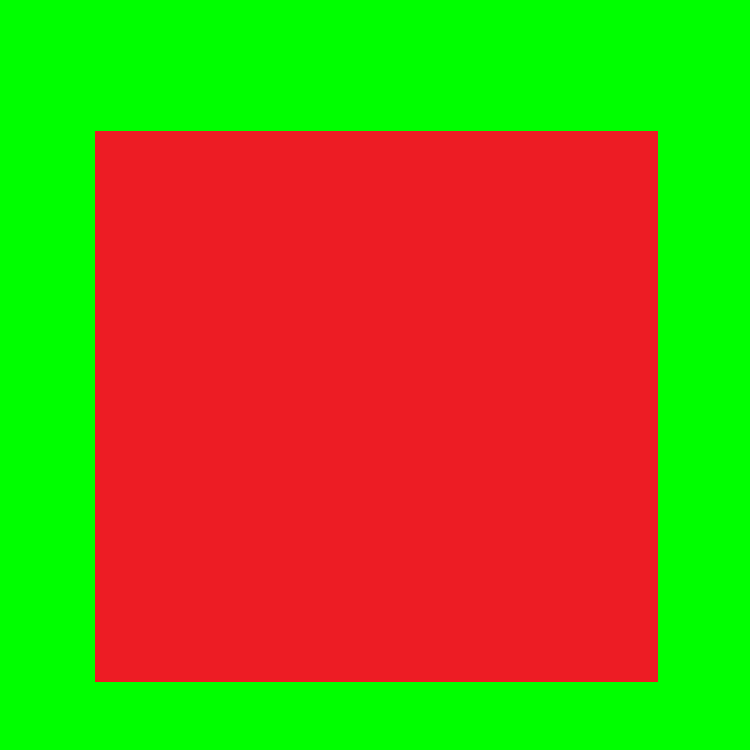
Max number of intersections - 29808. Just a bounding box - every pixel that intersects the bounding box intersects every triangle.

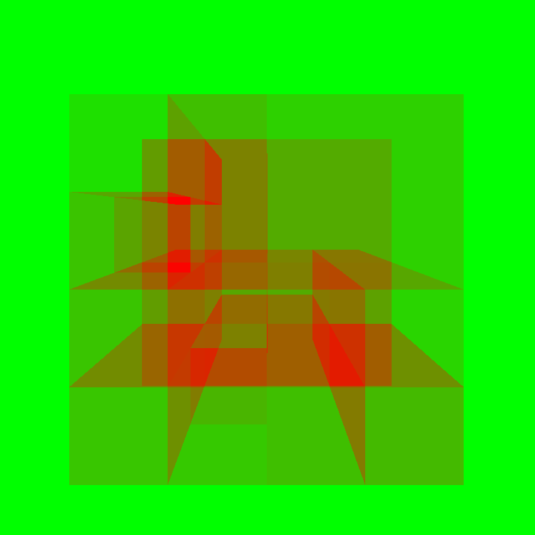
Max number of intersections - 7147. KD Tree with max 2000 triangles / node. You can vaguely see the global shape of the bunny

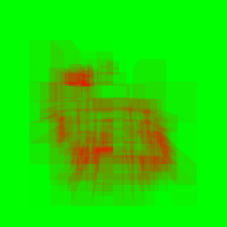
Max number of intersections - 1666. KD Tree with max 200 triangles / node. If you know it's supposed to be a bunny you can see it.

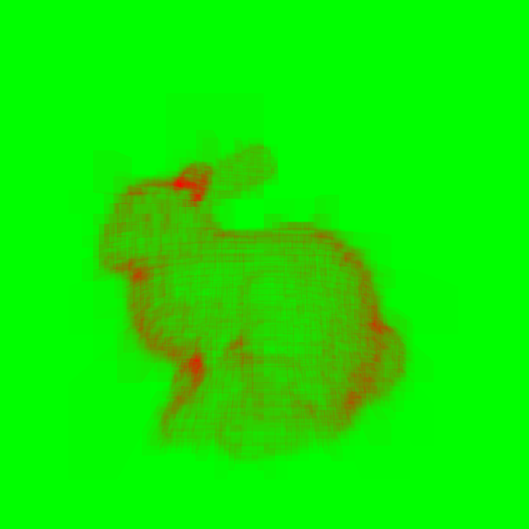
Max number of intersections - 467. KD Tree with max 20 triangles / node. Very few intersection test computed.

So we're only intersecting when we need to, which is a great thing.

###Stackless kd-tree traversal on the GPU

For this project, we implemented a stackless kd-tree on the GPU as discussed in "Stackless KD-Tree Traversal for High Performance GPU Ray Tracing" by Popov, Günther, Seidel, and Slusallek (2007). This method begins with a standard kd-tree, where each node maintains pointers to its children. To traverse such a tree requires recursion. Unfortunately, recursion is difficult to perform on the GPU. Instead, using methods introduced in the aforementioned paper, we convert our traditional kd-tree into a stackless kd-tree by adding something called a "rope structure".

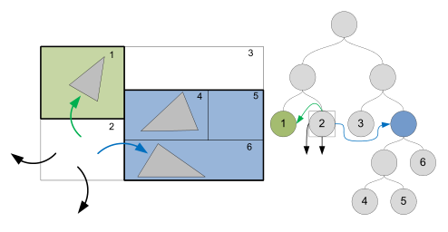
In the stackless kd-tree structure, every leaf node maintains a list of it's neighboring nodes through ropes. A rope is basically a pointer to another node in the tree. Each leaf node has six ropes, one for each face of its bounding boxes. These ropes are added as a post-process after initial kd-tree construction occurs.

During traversal, the first step is to set an entry and exit point for the ray into the kd-tree. Next, the tree is traversed from the root down in search of a "good" leaf node. This good leaf node is found by intelligently traversing child nodes by comparing the ray entry point into the current node's bounding box against the splitting plane value used to partition that space during kd-tree construction. Once a leaf node is reached, the triangles contained within that node are tested for intersection against the ray. If an intersection is found, then the exit point is updated to be the intersection point.

Regardless of whether or not an intersection occurs, the entry point into the next node is found by finding the ray exit point for the current node. This next node is a neighboring node connected to the current node via ropes. Once the bounding box face where the ray exit point exists is found, the rope connected to that face can be followed to the next node to be tested for triangle intersections. This algorithm terminates when the exit point becomes less than the entry point.

This traversal method is very efficient because thanks to ropes fewer nodes need to be traversed. Most importantly however, this traversal method can be implemented without recursion. The tree nodes can be packaged into an array where children and neighbors are represented by array indices. Such a stackless structure is ideal for a GPU computing environment.

You can read more about this method here.

###Performance analysis

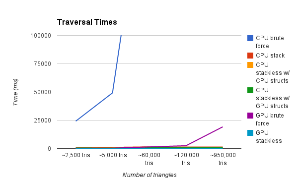
Now we're going to show some other performance statistics for the KD Tree.

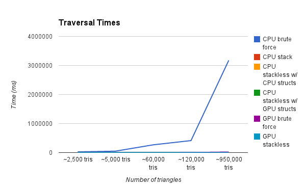
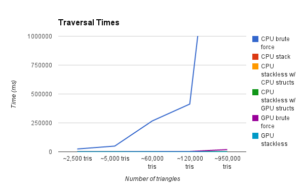
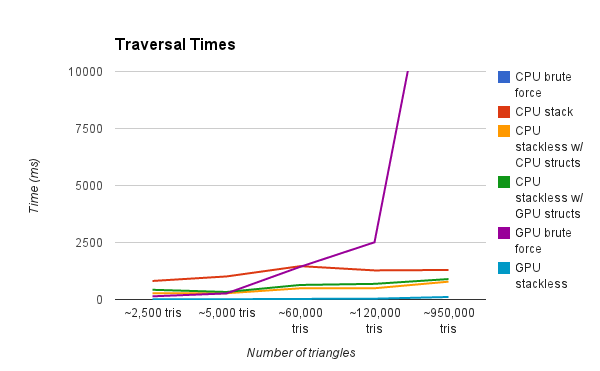
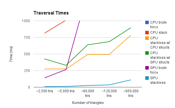
This graph is showing the render time of a scene with various amounts of triangles. Our test renders are a result of a simple raycasting operation where rays terminate after a single intersection. As you can see, the CPU Brute Force method is by far the slowest. We zoom in progressively on the graph to show further detail.

We also want to show the cost (in terms of percentage of compute) of the KD Tree construction as it relates to traversal.

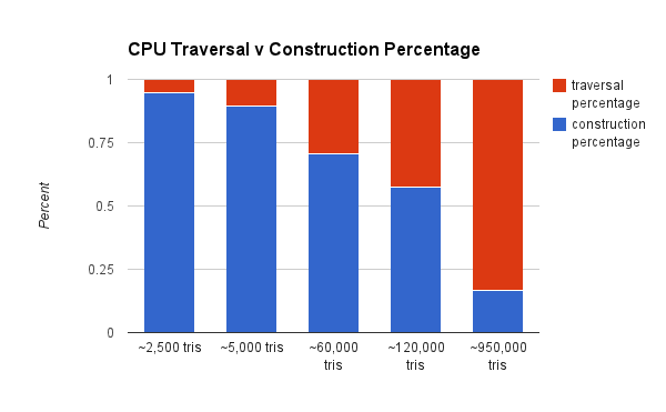
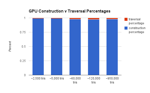
As you can see, the CPU construction is much less of a percentage of total compute. That's because the GPU has to incur the overhead of the additional port to the GPU. A GPU construction algorithm would rectify this.

Overall we're pretty happy with our results. We ended up spending a lot of time doing performance analysis and visualizations, which we had not done extensively before.

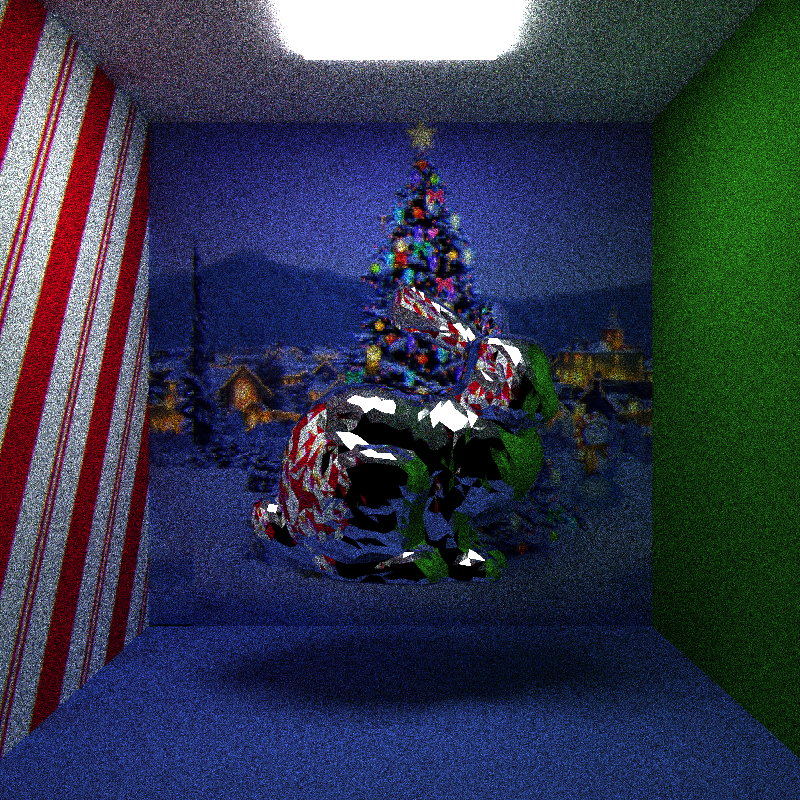
Path tracing with stackless kd-tree traversal on the GPU

This video demonstrates results after implementing stackless kd-tree traversal on the GPU into Danny's path tracer. Using this method, we were able to render 168 iterations of a 5000 triangle Stanford bunny mesh in 2 minutes with a ray trace depth of 10. For comparison, using a brute force approach on the GPU and the same scene, Danny's path tracer only managed to render 13 iterations in 2 minutes.

Here are some code samples that can be used to perform various kd-tree operations on both the CPU and GPU using our library.

To create a kd-tree with ropes for some input mesh and perform ray/mesh intersection testing using both stack and stackless traversal techniques:

#include "KDTreeCPU.h"

// obj_mesh <-- Mesh data structure

// Creates a traditional kd-tree, and also builds the rope structure for stackless traversal.
KDTreeCPU *kd_tree = new KDTreeCPU( obj_mesh->num_tris, obj_mesh->tris, obj_mesh->num_verts, obj_mesh->verts );

// Returns whether or not there was an intersection with the ray and the mesh the kd-tree was built around.
// Also returns t, hit_point, and normal,  which are the distance along the ray from the ray origin where the intersection occurred, the world-space intersection point, and the normal at the intersection point, respectively.
bool intersects = kd_tree->intersect( ray.origin, ray.dir, t, hit_point, normal );

// Equivalent functionality to previous intersection test, but traverses kd-tree in a stackless manner using rope structure.
bool intersects_stackless = kd_tree->singleRayStacklessIntersect( ray.origin, ray.dir, t, hit_point, normal );

To create a GPU-friendly stackless kd-tree for a mesh and perform ray/mesh intersection testing using this new GPU-friendly data structure:

#include "KDTreeGPU.h"

// kd_tree <-- CPU-friendly kd-tree data structure

KDTreeGPU *kd_tree_gpu = new KDTreeGPU( kd_tree );

// Create int array of triangle indices from GPU kd-tree int vector.
std::vector<int> tri_index_vector = kd_tree_gpu->getTriIndexList();
int *tri_index_array = new int[tri_index_vector.size()];
for ( int i = 0; i < tri_index_vector.size(); ++i ) {
    tri_index_array[i] = tri_index_vector[i];
}

bool intersects = cpuStacklessGPUIntersect( ray.origin, ray.dir, kd_tree_gpu->getRootIndex(), kd_tree_gpu->getTreeNodes(), tri_index_array, kd_tree_gpu->getMeshTris(), kd_tree_gpu->getMeshVerts(), t, hit_point, normal );

To perform stackless kd-tree traversal on the GPU:

#include "KDTraversalOnGPU.h"

// The following method can be executed on GPU devices and can be called from within CUDA kernels.
// Ray variables: ray_o, ray_dir.
// KDTreeGPU variables: root_index, tree_nodes, kd_tri_index_list.
// Mesh variables: tris, verts.
// Returns: t, hit_point, normal.
bool intersects = gpuStacklessGPUIntersect( const glm::vec3 &ray_o, const glm::vec3 &ray_dir, int root_index, KDTreeNodeGPU *tree_nodes, int *kd_tri_index_list, glm::vec3 *tris, glm::vec3 *verts, float &t, glm::vec3 &hit_point, glm::vec3 &normal );